Immune Cell Clustering
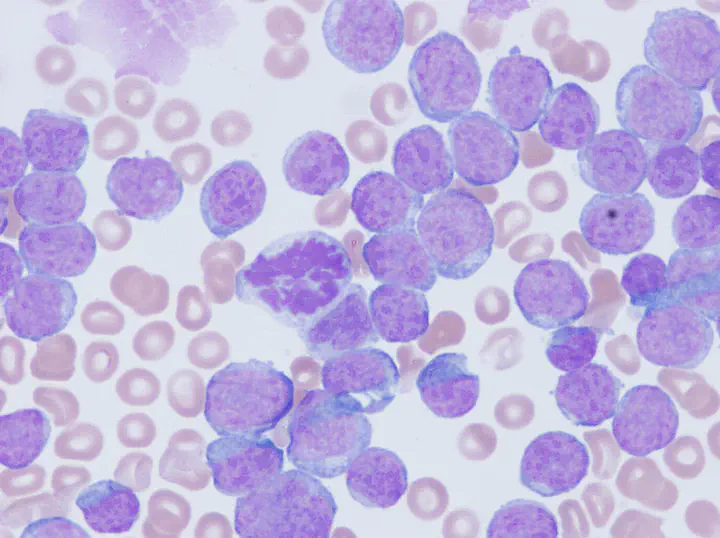 Peripheral blood smear1
Table of contents
- Background and motivation
- Getting started
- Data cleaning
- Data transformation
- PCA
- UMAP/tSNE
- Annotation
Background and motivation
Human peripheral blood mononuclear cells (PBMCs) are any blood cell with a round nucleus. PBMCs include lymphocytes (T cells, B cells, and NK cells), monocytes, and dendritic cells. In humans, the frequencies of these populations vary across individuals, but typically, lymphocytes are in the range of 70-90%, monocytes from 10-20%, while dendritic cells are rare, accounting for only 1–2%.
Most PBMCs are naïve or resting cells without effector functions. In the absence of an ongoing immune response T cells, the largest fraction of the isolated PBMCs, are mainly present as naïve or memory T cells. The naïve T-cells have never encountered their cognate antigen before and are commonly characterized by the absence of activation markers like CD25, CD44 or CD69 and the absence of the memory marker CD45RO isoform. Antigen recognition by a naïve T cell may result in activation of the cell, which will then enter a differentiation program and develop effector functions.2
Thus, we can differentiate the tissue microenvironment and understand its cellular composition by analyzing the biomarkers expressed through mRNA.
We will be working with a PBMC dataset from 10X Genomics, linked here. The dataset captures 2,700 single cells sequenced on the Illumina NextSeq 500. We want to cluster cells that are similar to each other, identify cluster biomarkers (differentially expressed features), and then assign cell types to the clusters.
Getting Started
We start by reading in the data. The Read10X() function reads in the output of the cellranger pipeline from 10X, returning a unique molecular identified (UMI) count matrix. The values in this matrix represent the number of molecules for each feature (i.e. gene; row) that are detected in each cell (column). We next use the count matrix to create a Seurat object. The object serves as a container that contains both data (like the count matrix) and analysis (like PCA, or clustering results) for a single-cell dataset.3
library(tidyverse)
library(patchwork)
library(Seurat)
library(BiocManager)
BiocManager::install("edgeR")

# Load the dataset
pbmc_data <- Read10X(data.dir = "/.../filtered_gene_bc_matrices/hg19/")
# Initialize the Seurat object with the raw data
pbmc <- CreateSeuratObject(counts = pbmc_data, project = "PBMC", min.cells = 1, min.features = 100)
Data Cleaning
Before proceeding to analyze the dataset, we must first clean it. We will filter cells based on common issues that arise in RNA sequencing and processing standards.
- Low-quality or dying cells may display excessive mitochondrial contamination. To filter these cells, we will determine the percentage of gene counts mapped to a reference genome. We use the set of all genes starting with MT- as a set of mitochondrial genes.
# Create a column in the Seurat object for percentage of mitochondrial genes mapped
pbmc[["MT_percent"]] <- PercentageFeatureSet(pbmc, pattern = "^MT-")
We need to set a threshold of cells – in this case, we will set it at 5% or greater mitochondrial counts.
- Droplets meant to capture, lyse, and tag single cells may be empty, may contain low-quality cells, or may contain multiple cells. The first two cases result in a low unique gene count, whereas the latter case results in a high unique gene count. Accounting for these errors requires us to filter the cells for outliers.
# Determine outliers with violin plot
VlnPlot(pbmc, features = c("nFeature_RNA", "nCount_RNA", "MT_percent"), ncol = 3)
We should filter cells that have unique gene counts less than 200 or over 2,500.
- The number of unique genes should correlate with the number of molecules detected per cell.
FeatureScatter(pbmc, feature1 = "nCount_RNA", feature2 = "nFeature_RNA")
As expected, there is a strong correlation between the gene count and molecular count. This result assures us that
Filtering the afore-mentioned cells:
pbmc <- subset(pbmc, subset = nFeature_RNA > 200 & nFeature_RNA < 2500 & MT_percent < 5)
Data Transformation \ 4 Now that the data has been cleaned, we can move on to transforming the data into more useful forms for analysis.
- In order to make accurate comparisions of gene expression between samples, we must normalize gene counts. The counts of mapped reads for each gene is proportional to the expression of mRNA (signal) in addition to many other factors (noise). Normalization is the process of scaling raw count values to account for the noise.
The most common factors to consider during normalization include:
-
Sequencing depth: Accounting for sequencing depth is necessary for comparison of gene expression between samples. In the example below, each gene appears to have doubled in expression in Sample A relative to Sample B, however this is a consequence of Sample A having double the sequencing depth.
-
Gene length: Accounting for gene length is necessary for comparing expression between different genes within the same sample. In the example, Gene X and Gene Y have similar levels of expression, but the number of reads mapped to Gene X would be many more than the number mapped to Gene Y because Gene X is longer.
-
RNA composition: A few highly differentially expressed genes between samples, differences in the number of genes expressed between samples, or presence of contamination can skew some types of normalization methods. Accounting for RNA composition is recommended for accurate comparison of expression between samples, and is particularly important when performing differential expression analyses.
In the example, if we were to divide each sample by the total number of counts to normalize, the counts would be greatly skewed by the DE gene, which takes up most of the counts for Sample A, but not Sample B. Most other genes for Sample A would be divided by the larger number of total counts and appear to be less expressed than those same genes in Sample B.
There are several normalization methods that account for some of these differences, but the one we will use is trimmed mean of M values (TMM). This method uses a weighted trimmed mean (the average after removing the upper and lower x% of the data) of the log expression ratios between samples. TMM accounts for all three factors, and can be used in gene count comparisons between and within samples.
# TMM Code
- We next calculate a subset of features that exhibit high cell-to-cell variation in the dataset (i.e, they are highly expressed in some cells, and lowly expressed in others). This is to distinguish true biological variability from the high levels of technical noise in single-cell experiments.5
Selection methods include (Seurat doc)
-
vst: First, fits a line to the relationship of log(variance) and log(mean) using local polynomial regression (loess). Then standardizes the feature values using the observed mean and expected variance (given by the fitted line). Feature variance is then calculated on the standardized values after clipping to a maximum (see clip.max parameter).
-
mean.var.plot (mvp): First, uses a function to calculate average expression (mean.function) and dispersion (dispersion.function) for each feature. Next, divides features into num.bin (deafult 20) bins based on their average expression, and calculates z-scores for dispersion within each bin. The purpose of this is to identify variable features while controlling for the strong relationship between variability and average expression.
# plot1 plot2 diff selection methods
- Next, we apply a linear transformation (‘scaling’) that is a standard pre-processing step prior to dimensional reduction techniques like PCA. The ScaleData() function:
- Shifts the expression of each gene, so that the mean expression across cells is 0
- Scales the expression of each gene, so that the variance across cells is 1 – This step gives equal weight in downstream analyses, so that highly-expressed genes do not dominate
The results of this are stored in pbmc[[“RNA”]]@scale.data
all.genes <- rownames(pbmc)
pbmc <- ScaleData(pbmc, features = all.genes)
References:
1 Mantle cell leukemia as a cause of leukostasis (Smith et. al)
2>/sup> https://www.ncbi.nlm.nih.gov/books/NBK500157/#:~:text=PBMCs%20include%20lymphocytes%20(T%20cells,for%20only%201%E2%80%932%20%25.
3 https://satijalab.org/seurat/articles/pbmc3k_tutorial.html#assigning-cell-type-identity-to-clusters
4 https://hbctraining.github.io/DGE_workshop/lessons/02_DGE_count_normalization.html
5 https://www.nature.com/articles/nmeth.2645